Analyze with Iceberg, Serve with Lance: a Two-Format Lakehouse on SeaweedFS

Two table formats have become popular for two very different jobs. Apache Iceberg owns analytics: columnar scans, partition pruning, SQL aggregations — “average score by category across the whole table.” Lance (the format behind LanceDB) owns the opposite access pattern: random-access point lookups and vector similarity search — “give me the 5 documents most like this one.” Iceberg handles that second query poorly, because Parquet is optimized for column projection and predicate pushdown, not fetching individual rows; Lance is built for it, with ~100× faster random access and a native vector index.

So the emerging best practice for AI data isn’t to pick one — it’s to run both, co-located in object storage, with a SQL engine bridging them (Merced, Lance and Iceberg for Multimodal AI Data). Iceberg holds the structured, governed source of truth; Lance holds the embeddings and serves retrieval; DuckDB joins across the two without an ETL step in between.

SeaweedFS table buckets make that architecture a single deployment. One SeaweedFS cluster serves an Iceberg table bucket and a Lance table bucket from the same S3 object store, each with its built-in catalog. This post runs the whole workflow end to end on one machine — analyze a document catalog in Iceberg, derive embeddings, serve fast lookups from Lance, and join the two in DuckDB. Nothing is hand-waved: every command and output block below is a real capture.

Start SeaweedFS with both buckets

One weed mini runs both catalogs. Create an Iceberg bucket lake and a Lance bucket vec in a single flag — a bucket name takes an optional :FORMAT suffix (default ICEBERG):

weed mini -dir=./data -s3.config=s3config.json -tableBucket=lake,vec:LANCE

Both catalogs come up over the same S3 endpoint:

    S3 Endpoint:     http://localhost:8333
    Iceberg Catalog: http://localhost:8181
    Lance Namespace: http://localhost:9101

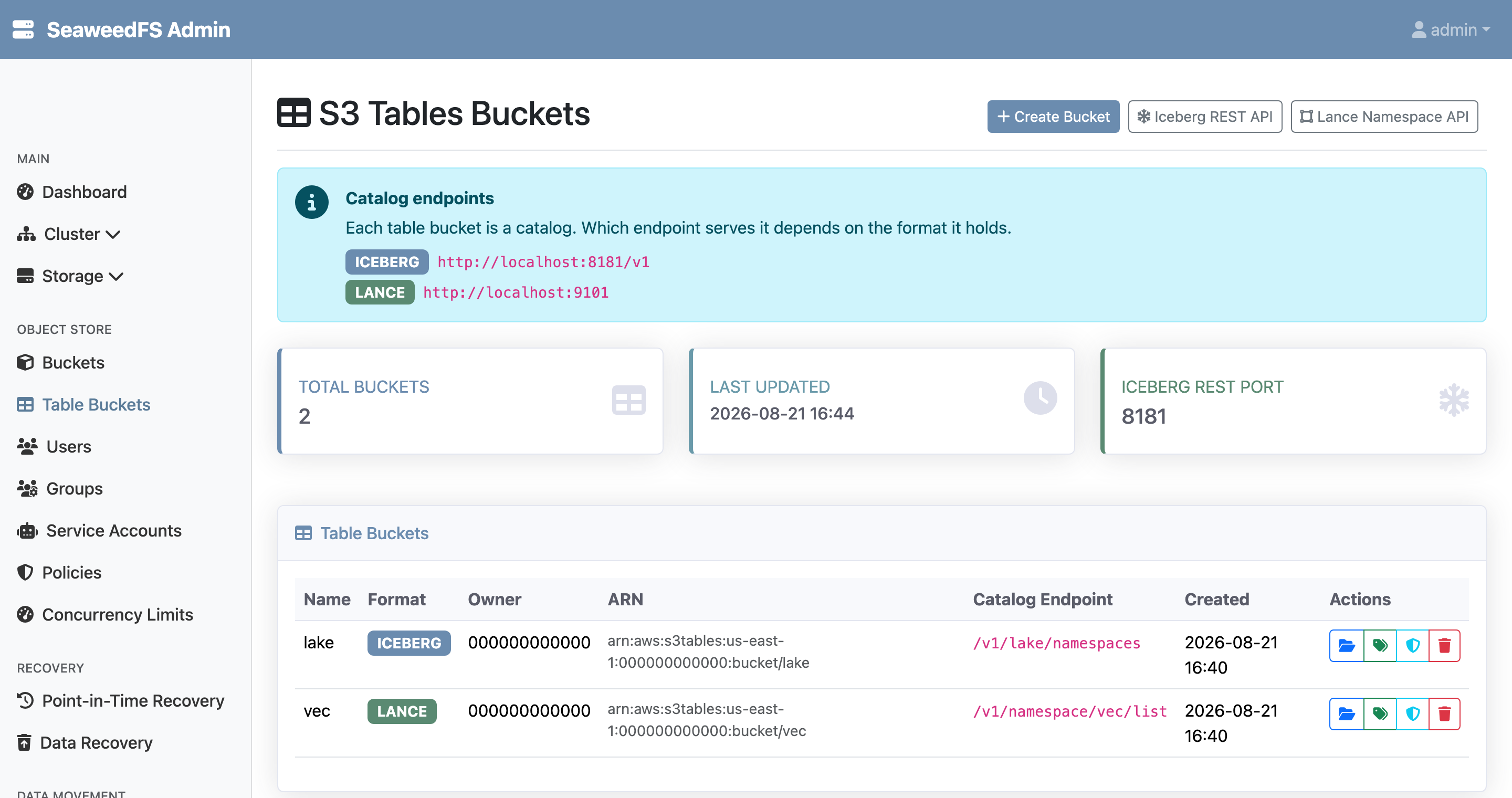
The Admin UI’s Table Buckets page shows the two side by side — same store, different format, different catalog endpoint:

Install the clients — one environment covers the whole workflow (s3config.json holds an S3 identity; use its access key / secret below):

pip install "pyiceberg[pyarrow]" lancedb lance-namespace pylance duckdb numpy

All the Python below shares this setup (the same credentials work for both catalogs and the S3 data):

AK = "AKIAIOSFODNN7EXAMPLE"
SK = "wJalrXUtnFEMI/K7MDENG/bPxRfiCYEXAMPLEKEY"
storage = {"aws_endpoint": "http://localhost:8333", "allow_http": "true",
           "aws_access_key_id": AK, "aws_secret_access_key": SK, "aws_region": "us-east-1"}

Step 1 — Land the data in Iceberg, and analyze it

Iceberg is the source of truth. Write a document catalog into it with PyIceberg — id, title, category, a quality score, and a publish time:

import datetime, random, pyarrow as pa
from pyiceberg.catalog.rest import RestCatalog

MIX = (["databases"]*30 + ["ml"]*25 + ["systems"]*20 + ["security"]*15 + ["networking"]*10)
rng, base = random.Random(7), datetime.datetime(2026, 8, 21, 12, 0)
rows = {"id": [], "title": [], "category": [], "score": [], "published": []}
for i in range(1200):
    c = MIX[i % len(MIX)]
    rows["id"].append(i); rows["category"].append(c); rows["title"].append(f"{c} note {i}")
    rows["score"].append(round(rng.random(), 3))
    rows["published"].append(base - datetime.timedelta(days=(i*13) % 90, minutes=i))
data = pa.table(rows, schema=pa.schema([
    ("id", pa.int64()), ("title", pa.string()), ("category", pa.string()),
    ("score", pa.float64()), ("published", pa.timestamp("us"))]))

lake = RestCatalog(name="lake", uri="http://localhost:8181", warehouse="s3://lake",
                   credential=f"{AK}:{SK}",
                   **{f"s3.{k}": v for k, v in {
                       "endpoint": "http://localhost:8333", "path-style-access": "true",
                       "access-key-id": AK, "secret-access-key": SK, "region": "us-east-1"}.items()})
lake.create_namespace_if_not_exists("docs")
lake.create_table_if_not_exists("docs.catalog", schema=data.schema).append(data)

Now analyze it with DuckDB, attached to the Iceberg REST catalog. This is Iceberg’s home turf — scan the whole table and aggregate:

import duckdb
con = duckdb.connect()
con.execute("INSTALL iceberg; LOAD iceberg;")
con.execute(f"CREATE SECRET ice (TYPE ICEBERG, CLIENT_ID '{AK}', CLIENT_SECRET '{SK}', OAUTH2_SERVER_URI 'http://localhost:8181/v1/oauth/tokens')")
con.execute(f"CREATE SECRET s3 (TYPE S3, KEY_ID '{AK}', SECRET '{SK}', ENDPOINT 'localhost:8333', URL_STYLE 'path', USE_SSL false)")
con.execute("ATTACH 's3://lake' AS lake (TYPE ICEBERG, ENDPOINT 'http://localhost:8181', SECRET ice)")

con.sql("""SELECT category, count(*) AS docs, round(avg(score), 3) AS avg_score
           FROM lake.docs.catalog GROUP BY category ORDER BY docs DESC""").show()

┌────────────┬───────┬───────────┐
│  category  │ docs  │ avg_score │
├────────────┼───────┼───────────┤
│ databases  │   360 │     0.472 │
│ ml         │   300 │     0.498 │
│ systems    │   240 │     0.506 │
│ security   │   180 │      0.45 │
│ networking │   120 │     0.475 │
└────────────┴───────┴───────────┘

Filter it down to a working set with plain SQL — high-quality, recent docs:

con.sql("""SELECT count(*) AS working_set FROM lake.docs.catalog
           WHERE score >= 0.8 AND published >= TIMESTAMP '2026-07-01'""").show()

┌─────────────┐
│ working_set │
│         136 │
└─────────────┘

Step 2 — Derive embeddings and write them to Lance

Read the docs back through DuckDB, compute an embedding per document, and write a Lance table into the vec bucket. Lance’s catalog (the Lance Namespace) records where the table lives; the vectors are written straight to S3.

import numpy as np, lance, lance_namespace as ln
DIM = 16
docs = con.sql("SELECT id, category, score FROM lake.docs.catalog ORDER BY id").fetch_arrow_table()
ids, cats, scores = (docs.column(c).to_pylist() for c in ("id", "category", "score"))

# Stand-in embeddings: one fixed vector per category + a little per-doc jitter, so
# same-topic docs land near each other. Swap in CLIP / BGE / an API model for real text.
crng = np.random.default_rng(0)
centers = {c: (lambda v: v/np.linalg.norm(v))(crng.normal(size=DIM))
           for c in ["databases", "ml", "systems", "security", "networking"]}
def embed(doc_id, cat):
    v = centers[cat] + np.random.default_rng(1000 + doc_id).normal(scale=0.15, size=DIM)
    return (v / np.linalg.norm(v)).astype(np.float32)
vecs = [embed(i, c) for i, c in zip(ids, cats)]

lance_tbl = pa.table({"id": pa.array(ids, pa.int64()), "category": pa.array(cats),
                      "score": pa.array(scores, pa.float64()),
                      "vector": pa.array([v.tolist() for v in vecs], pa.list_(pa.float32(), DIM))})
ns = ln.connect("rest", {"uri": "http://localhost:9101"})
ns.create_namespace(ln.CreateNamespaceRequest(id=["vec"], mode="EXIST_OK"))
ns.create_namespace(ln.CreateNamespaceRequest(id=["vec", "docs"], mode="EXIST_OK"))
loc = ns.declare_table(ln.DeclareTableRequest(id=["vec", "docs", "embeddings"])).location
lance.write_dataset(lance_tbl, loc, storage_options=storage, mode="overwrite")

lance: wrote 1200 embeddings to s3://vec/docs/embeddings

Step 3 — Fast lookups from Lance

Two things Lance does that Iceberg can’t do cheaply. First, random-access point lookups — fetch specific rows by position, no scan:

lance.dataset(loc, storage_options=storage).take([7, 250, 999], columns=["id", "category"]).to_pylist()

[{'id': 7, 'category': 'databases'}, {'id': 250, 'category': 'ml'}, {'id': 999, 'category': 'networking'}]

Second, vector search. Build an ANN index and find the nearest neighbours of a document:

import lancedb
db = lancedb.connect_namespace("rest", {"uri": "http://localhost:9101"}, storage_options=storage)
t = db.open_table("embeddings", namespace_path=["vec", "docs"], storage_options=storage)
t.create_index(metric="cosine", vector_column_name="vector",
               index_type="IVF_PQ", num_partitions=4, num_sub_vectors=4)

hits = t.search(vecs[42].tolist()).limit(6).to_list()   # doc 42 is an "ml" note
print([(h["id"], h["category"]) for h in hits if h["id"] != 42][:5])

[(145, 'ml'), (151, 'ml'), (1147, 'ml'), (1130, 'ml'), (37, 'ml')]

Every neighbour is an ml doc — the clustered embeddings behave the way a good index should. (IVF_PQ is approximate, so your exact ids and order may differ.)

Step 4 — The bridge: join Lance and Iceberg in one query

The neighbours are just ids and distances. The meaning — titles, categories, scores, business rules — lives in Iceberg. Because both are reachable from the same DuckDB session, one SQL statement joins across the two formats, no ETL:

neighbours = pa.table({"id": pa.array([h["id"] for h in hits if h["id"] != 42][:5], pa.int64()),
                       "distance": pa.array([round(h["_distance"], 4) for h in hits if h["id"] != 42][:5])})
con.register("neighbours", neighbours)

con.sql("""SELECT n.id, n.distance, c.title, c.category, c.score
           FROM neighbours n JOIN lake.docs.catalog c ON c.id = n.id
           ORDER BY n.distance""").show()

┌───────┬──────────┬──────────────┬──────────┬────────┐
│  id   │ distance │    title     │ category │ score  │
├───────┼──────────┼──────────────┼──────────┼────────┤
│   145 │   0.2995 │ ml note 145  │ ml       │  0.484 │
│   151 │   0.3141 │ ml note 151  │ ml       │  0.161 │
│  1147 │   0.3369 │ ml note 1147 │ ml       │  0.523 │
│  1130 │   0.3414 │ ml note 1130 │ ml       │  0.745 │
│    37 │   0.3457 │ ml note 37   │ ml       │  0.428 │
└───────┴──────────┴──────────────┴──────────┴────────┘

And because it’s SQL, a business filter fuses with the vector search in the same statement — keep only the decent-quality neighbours:

con.sql("""SELECT n.id, n.distance, c.title, c.score
           FROM neighbours n JOIN lake.docs.catalog c ON c.id = n.id
           WHERE c.score >= 0.5
           ORDER BY n.distance""").show()

┌───────┬──────────┬──────────────┬────────┐
│  id   │ distance │    title     │ score  │
├───────┼──────────┼──────────────┼────────┤
│  1147 │   0.3369 │ ml note 1147 │  0.523 │
│  1130 │   0.3414 │ ml note 1130 │  0.745 │
└───────┴──────────┴──────────────┴────────┘

That’s “similar and high-quality” — vector retrieval from Lance, the quality gate and the human-readable metadata from Iceberg, resolved in one query.

Why one SeaweedFS makes this simple

• One object store, two formats. The Iceberg tables and the Lance datasets are plain objects in the same SeaweedFS cluster. No second system to run for vectors, no copy between a warehouse and a vector database.
• Two built-in catalogs, one set of credentials. The Iceberg REST catalog (:8181) and the Lance Namespace (:9101) authenticate with the same S3 keys. DuckDB attaches the Iceberg catalog; lance/LanceDB reach the Lance one; both read data directly from the S3 endpoint.
• DuckDB is the bridge. It queries Iceberg through the catalog and Lance results as Arrow, so a single JOIN spans both — the “SQL bridge” the multimodal-lakehouse pattern calls for.
• Same durability for both. Vectors, indexes, and Iceberg data files all inherit SeaweedFS replication, erasure coding, and cloud tiering.

One honest note: the embeddings here are a deterministic stand-in so the walkthrough needs no model download. In production you’d write real embeddings (CLIP, BGE, an API model) into the same Lance table — the plumbing is identical.

Further reading: Lance and Iceberg for Multimodal AI Data · the Lance format · Apache Polaris and Lance.

More on SeaweedFS table buckets: what they are · querying with DuckDB · running ClickHouse · vector search with LanceDB.